
In the last post I mentioned a need to add video sync to really hit our rolling shutter effect out of the park. I have an eval board coming for an HDMI decoder/encoder pair, but had a little time on Monday so I went ahead and fleshed what is sometimes called a “transform”, the ability to position, scale, and rotate an image we are projecting.
Compared to a modern first person shooter game…

What we are going to do is pretty simple. Still, the first time I was shown a linear algebra rotation matrix in the early 80s I thought it was magic, and the feeling has never completely gone away.
There are a fair number of textbooks and tutorials floating around, but for our purposes it starts with trigonometry, the wonderful world of right triangles. Although it is undoubtedly not PC, I still remember the trig relationships with “I can measure the circumference of the earth with this stick, a tape measure, and my good buddy SOH CAH TOA!” It turns out you can’t, at least not super accurately, because the earth is not really a sphere, but in the world of vector laser graphics, SOH CAH TOA is, indeed, our good friend!
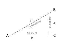
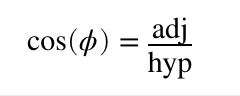
In the mnemonic, S, C, and T stand for sine, cosine, and tangent. O, H, and A stand for opposite, adjacent, and hypotenuse. The basic idea is that if you divide the lengths of two of the triangle’s three sides, you will get a specific ratio, and that ratio always represents the same angle. For example, the cosine of angle A above is the length of the adjacent (b) divided by the length of the hypotenuse (c). Or, CAH for short:
This is also our first laser rotation.
The cosine for zero degrees is one. This is pretty easy to visualize with our triangle above. If b/c = 1, then b and c are the same length, making angle A = 0 degrees.
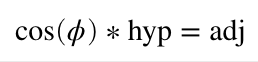
Now that you have a flat triangle in your mind, pretend it is our laser projection viewed from above. The hypotenuse is a line in our graphic ending at coordinate {c, 0} (where the hypotenuse meets B). We want to rotate it around our Y axis (at connection A). We know the length of our hypotenuse (c) because we have an X coordinate, and we know the angle we want for rotation. Since we have two parts of CAH, we can rearrange the formula above and solve for the part we don’t have:
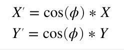
If we want to rotate 45 degrees, cosine is approximately 0.707, so our new coordinate is {0.707*c, 0}
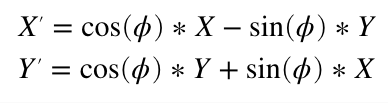
Rotating around the X axis is very similar. We just use the cosine of the desired angle to scale our Y coordinate instead of X. This means that if we only wanted to rotate around the X and Y axes, we’d only need two multiplies and our formula would look like this:
Rotating around the Z axis, the line coming towards us, is a bit more complicated. I’m not going to duplicate one of the many tutorials online, but you can work it out very much like above (hint, thinking about two triangles always helps me) and you should end up with a Z rotation formula something like this:
Instead of a formula, we can express this as a linear algebra matrix. Z rotation is:
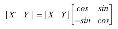
When you multiple two matrixes together you “multiply and accumulate”. Basically multiplying and adding horizontal rows from the left operand with vertical columns from the right operand.
So the matrix above is the same basic steps as the four multiplies and two adds (we use a negative value to get a subtract) from the Z rotate formula we derived earlier. What makes the matrix magic is two things. First, most the operations we are interested in can be expressed by one. For example:
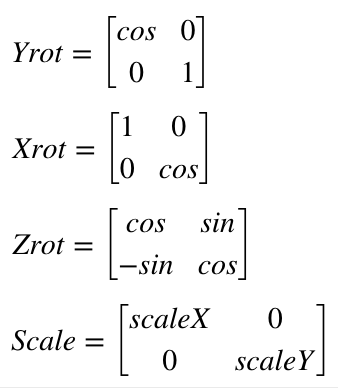
Second, you can combine them. Matrix multiplication is not commutative. That is, A*B will generally not give the same answer as B*A, but you can typically combine rotation and transform matrixes, provided you multiply things in the right order. So we could multiply the operation matrixes by each other and derive a single matrix. Then do all those operations on each point in our image with the same four multiplies and two additions as our Z rotation above. Like I said, magic!
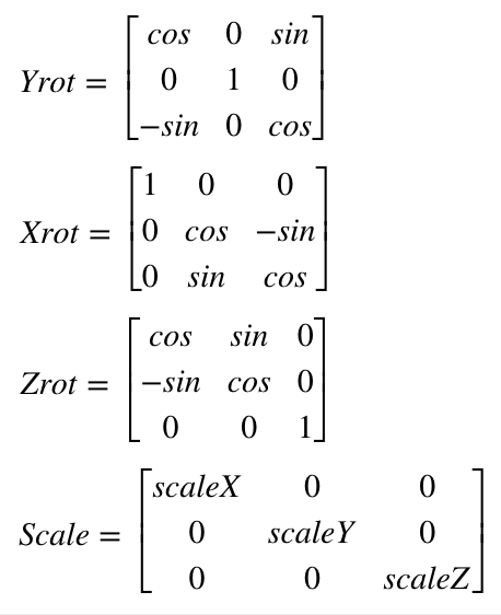
If you read a tutorial on this subject they will not normally use a 2×2 matrix, but something called homogenous coordinates and a 3×3 matrix for 2D graphics. This lets you do things like position the image as well. But we won’t mess with that until we address things like perspective later. For now we will just stick with a simple rotational matrix. However, we will expand to 3×3 to accommodate 3D graphics, since ILDA images can contain a Z position for each coordinate as well. If you worked out 2D Z rotation for yourself above, you won’t be surprised to see that our matrixes for 3D look like this:
Now that we have an idea what we want to do, we have to pick a way to code it. As it happens, we have two really good possibilities with our STM32F769 MCU. The ARM core has something called the DSP instructions and this chip has a double precision floating point unit (FPU). There are pros and cons to both approaches.
The DSP instructions are very fast (multiply and accumulate in a single instruction that executes in a single clock cycle), but it is integer math (whole numbers only). So you usually have to scale operators up and down and give some thought to your target ranges. Math library support for the DSP instructions is also a bit sketchy, at least on the free tools we are using. We might still end up back here, but to get things going I went with the double precision FPU to start.
To use the FPU, the first thing we have to do is tell the compiler we want to. Those options are stashed away in Project Settings / C/C++ Build / Settings / Target Processor:

“Float ABI” has to be set to use FP instructions (Hardware) and the FPU type has to be set to the one on our MCU (harder to lookup than you might think). In addition to telling the compiler to use it, like many peripherals on our MCU, the FPU also has to be enabled. This already conditionally happens in an existing function called SystemInit():
  /* FPU settings ------------------------------------------------------------*/
  #if (__FPU_PRESENT == 1) && (__FPU_USED == 1)
    SCB->CPACR |= ((3UL << 10*2)|(3UL << 11*2));  /* set CP10 and CP11 Full Access */
  #endif
With hardware floating support on, the next thing to do is to take a stab at our first implementation of a transform as a structure we can apply as we scan:
typedef struct {
	int32_t posX;			// X, Y position
	int32_t posY;
	int32_t roX;			// Rotation offset
	int32_t roY;
	int32_t roZ;
	int32_t blankOffset;	        // Blanking/Color offset
	double intensity;		// Intensity (0-1)
	double scaleX;			// X,Y, and Z scale (0-2)
	double scaleY;
	double scaleZ;
	double matrix11;		// 3x3 Rotation Matrix
	double matrix12;
	double matrix13;
	double matrix21;
	double matrix22;
	double matrix23;
	double matrix31;
	double matrix32;
	double matrix33;
} TRANSFORM;
Again, this is really just a placeholder. We will probably make a matrix type at some point, and we’ll eventually want to transform color as well, etc. But this is good enough for a test.
We can position, rotate, scale, control intensity, and add a rotation offset, which I’ll explain shortly. We can also adjust the blanking/color offset. You may recall that I mentioned that graphics from different eras were created with different assumptions about the speed of the blanking and coloring mechanisms. Up to now we’ve been hardcoding a shift for very old graphics played faster than they were originally intended. Now we can change that on a frame by frame basis.
Using all these settings our scan interrupt handler has gotten a bit longer, but is still pretty clear. It still isn’t optimized. But at this point that actually helps:
void TIM2_IRQHandler()
{
if (TIM2->SR & TIM_SR_UIF)
{
TIM2->SR &= ~TIM_SR_UIF;
// Latch the previous values
HAL_GPIO_WritePin(GPIOA, GPIO_PIN_11, GPIO_PIN_SET);
ILDA_FORMAT_4 *pntData;
pntData = &(CurrentFrame->points);
int32_t val;
double d;
double dx, dy, dz;
uint8_t clip = 0;
dx = pntData[curPoint].x.w;
dx *= currentTransform.scaleX;
dx += currentTransform.roX;
dy = pntData[curPoint].y.w;
dy *= currentTransform.scaleY;
dy += currentTransform.roY;
dz = pntData[curPoint].z.w;
dz *= currentTransform.scaleZ;
dz += currentTransform.roZ;
d = dx * currentTransform.matrix11 + dy * currentTransform.matrix12 + dz * currentTransform.matrix13;
val = (int32_t)d;
val += currentTransform.posX;
if (val < -32768)
{
val = -32768;
clip = 1;
}
if (val > 32767)
{
val = 32767;
clip = 1;
}
val += 32768;
DacOut[7] = val >> 8;
DacOut[8] = val & 0xFF;
d = dx * currentTransform.matrix21 + dy * currentTransform.matrix22 + dz * currentTransform.matrix23;
val = (int32_t)d;
val += currentTransform.posY;
if (val < -32768)
{
val = -32768;
clip = 1;
}
if (val > 32767)
{
val = 32767;
clip = 1;
}
val += 32768;
DacOut[5] = val >> 8;
DacOut[6] = val & 0xFF;
int16_t idx;
if (CurrentFrame->numPoints > (uint32_t)abs(currentTransform.blankOffset))
{
idx = curPoint + currentTransform.blankOffset;
if (idx < 0)
idx += CurrentFrame->numPoints;
else if (idx >= (int16_t)CurrentFrame->numPoints)
idx -= CurrentFrame->numPoints;
}
else
idx = curPoint;
if ((pntData[idx].status & 0x40) || clip)
{
DacOut[3] = DacOut[4] = 0;
DacOut[1] = DacOut[2] = 0;
DacOut[15] = DacOut[16] = 0;
}
else
{
double i;
i = pntData[idx].red * currentTransform.intensity;
DacOut[3] = (uint8_t)i;
i = pntData[idx].green * currentTransform.intensity;
DacOut[1] = (uint8_t)i;
i = pntData[idx].blue * currentTransform.intensity;
DacOut[15] = (uint8_t)i;
}
if (pntData[curPoint].status & 0x80)
{
curPoint = 0;
// Is it time for a new frame?
if (NewFrameRequest)
{
CurrentFrame = NewFrame;
NewFrameRequest = 0;
}
// Update transform?
if (UpdateTransform)
{
memcpy (¤tTransform, &pendingTransform, sizeof(TRANSFORM));
UpdateTransform = 0;
}
}
else
++curPoint;
HAL_GPIO_WritePin(GPIOA, GPIO_PIN_11, GPIO_PIN_RESET);
HAL_SPI_Transmit_DMA(&Spi_Handle, (uint8_t*) DacOut, sizeof(DacOut));
}
}
Our processing pipeline is slightly more complicated than the single matrix we described above. It’s broken down into a few steps:
- Apply scale to the X, Y, and Z coordinates
- Add X, Y, and Z rotational offset
- Apply the rotation matrix
- Add position
- Check for clipping
The pros and cons of these decisions are a big subject I don’t really want to go into now. But we will be revisiting this again fairly soon. For now, let’s just call this Laser Bling 101. The first big question is, does it work? Thankfully, the answer is yes:
This flag graphic isn’t great, but it is the only ILDA file with Z values in it I have, and you can see that we are rotating in 3D as we rotate this frame around the X axis. Here is the same 3D image animating and rotating around both the X and Z axes:
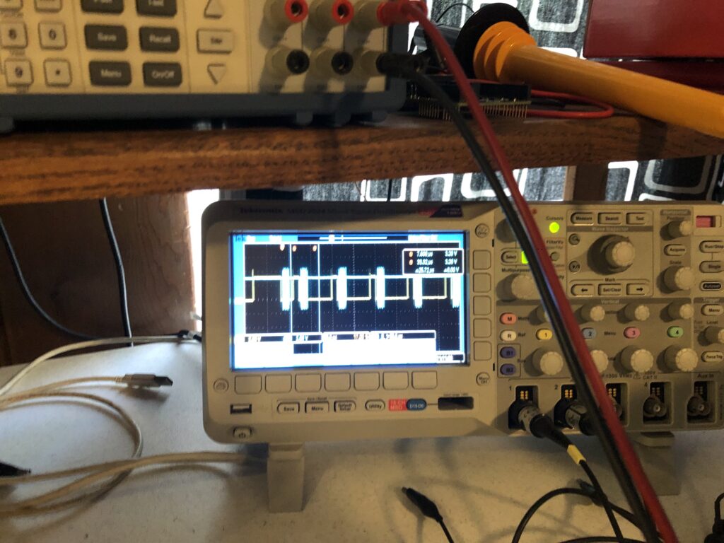
The next question is, how is performance? I’d say, not bad at all. Better than I expected without some optimizations, to be honest:
We are using about 16% of the CPU time to scan at 30 kHz, and we still have quite a bit of room for improvement. Now let’s take a quick look at the other parts of the transform.
Intensity lets us crank down to 10% so that white images don’t freak out the camera on my phone. We can then scale our favorite sax playing pig down and spin him on the Z axis:
He isn’t quite drawn centered, but is sort of rotating around his center of mass. We could add a little rotational offset to center him up, but let’s add a little bigger positive roY. Now he is rotating around his feet:
If we invert the polarity of the roY, he is rotating around his head:
Positioning lets us shift the whole thing around the available scan angle. If we move too far, the image will clip:
There are a couple schools of thought on how to handle clipping. One is to not scan the clipped points in images. This frees up scan time for other images, making those other images brighter. But we are still going to want to lock to rolling shutters, so we scan the clipped points so there is no time shift, but we blank them out so any squishing or distortion isn’t visible.
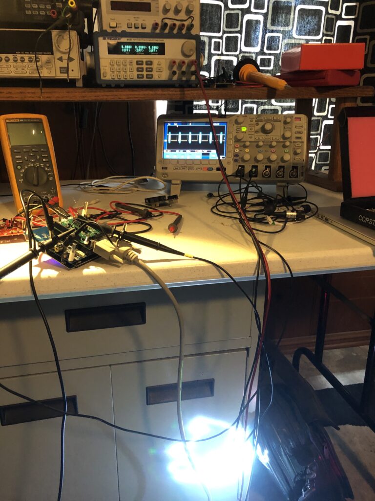
There is a consideration for performance I should touch on. Building our rotation matrix is more intensive than using it. It takes 54 multiplies to combine the X, Y, and Z rotation matrices. That’s not terrible. We typically only need to update the matrix 10 to 30 times per second, not the 30,000 times a second (or more) we use the combined matrix for scanning. But look what happens when I try calling sin() and cos() one time each at the end of each graphic frame:
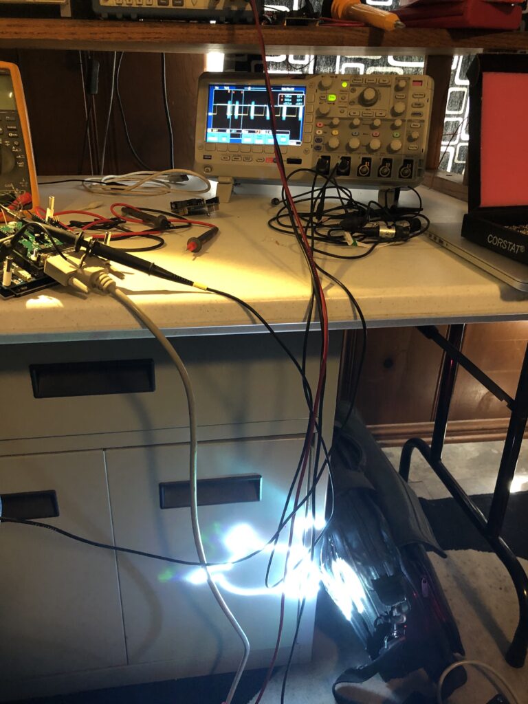
If we zoom in on the scope we can see that those two calls push our processor utilization to almost 100% for that one scan interval:
If you look at the library source code for, say, sin() you will find it is very complex. It uses one algorithm if you are very close to 0 degrees, basic Taylor series calculations out to a couple of degrees, and then multiple calculations applied to correction tables when the angles get larger.
We aren’t going to do that. I pre-calculated a sine table in 0.1 degree steps and stored the results in flash memory as a lookup table. We don’t need a separate table for cosine because we just need to shift 90 degrees in our sine table to get cosine for the same angle:
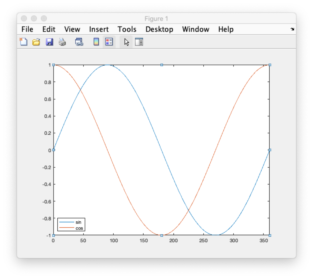
Going in 0.1 degree steps might seem like overkill, but it gives us more granularity of control in terms of rotation speed and will let us make smoother transitions as we start and stop rotations. If we end up needing even more granularity we have the room for it in flash memory but, for now, rotations are very smooth:
That’s enough for now. Sorry this post was so long. Depending on when the eval card arrives we will either be testing HW sync operations next, or putting together our first host control application.
Update: HW sync it is!
Leave a Reply