In the last post we sketched out our basic Arduino Uno compatible “shield” board for ILDA projector control. I then indicated that I would start converting that sketch into a proper schematic next. I did begin that process, but when I work on hardware designs I try to also give some thought to how software/firmware will interact with it.
I have used the TI DAC discussed last time in another project and knew that the speed and output quality were on par with what I wanted, but I didn’t like how the interface with our selected control board was shaping up.
The problem is the implementation of SPI (‘Serial Peripheral Interface’) on each chip. The ST MCU’s onboard SPI controllers are pretty good. You can setup the peripheral to output memory directly via DMA (Direct Memory Access) and there is even hardware support for CRC (Cyclic Redundancy Check) error checking. The Achille’s heel is the ‘NSS’ line. NSS stands for “Negative (Active Low) Slave Select”. Basically, this line signals a slave device when it should receive data.
The ST SPI peripheral can drive the NSS line automatically, but only for packets of either 1 or 2 bytes in length. But the TI DAC I selected uses a 3 byte packet. So we would have to use the NSS line in software controlled mode.
Further, if we look at the operating modes of the TI DAC, the only one really suitable for our purposes is ‘stand alone’:
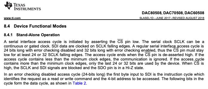
In this mode we have to write to each of the 8 DACs individually and control NSS (connected to the /CS pin on the DAC chip) via software each time. That’s a lot of firmware overhead managing an I/O line just so we can update our DAC values. There are some ways we could work around this with some hardware tweaking, but all the ones that I could think of involved modifying the MCU board to use other peripherals and pins, so I started thinking about DAC alternatives. As it happens, I’ve been working with another TI DAC on a work project, a DAC81408. I even happen to have the TI EVM (Evaluation Module) for it!
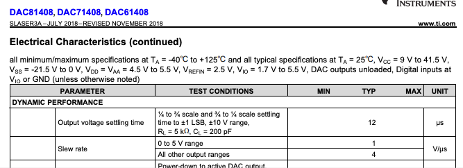
But I had two concerns about moving to the DAC81408. First, it is about $15 more expensive in small quantities than the DAC80508. Not the end of the world, but something to keep in mind. Second, the spec’ed settle time is 2.5x longer (12 uS vs 5 uS):
As a rule of thumb, a settle time at least two times faster than your max sample rate is a good starting point. 1 / 0.000005 = 200,000, more than 3x our max sample rate of 60,000. But 1/ 0.000012 = 83,333, just barely 1x our max. But the DAC81408 has some very wide output ranges (ex. +/- 20V) that can be selected, and settle time would be worse on an amplifier at those gains, so it was not clear how the DAC would perform for our application.
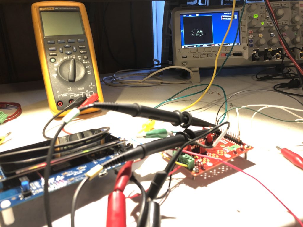
Fortunately, the EVM board has just two chips on it, the TI DAC and an external reference chip we aren’t using:
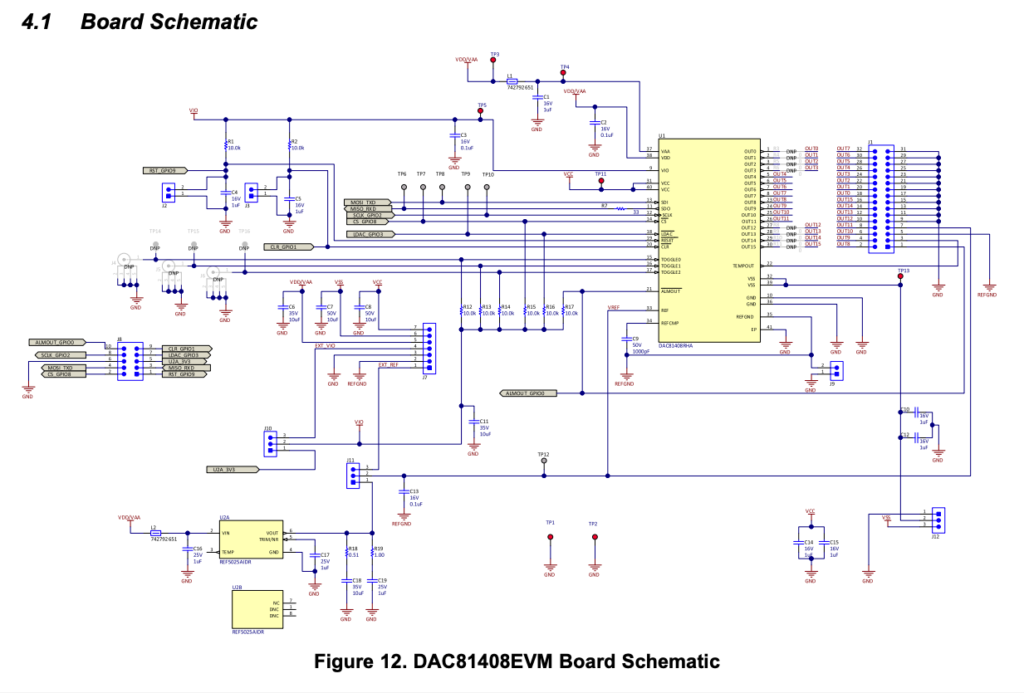
There is also a handy connector for accessing the critical signals we need:
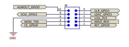
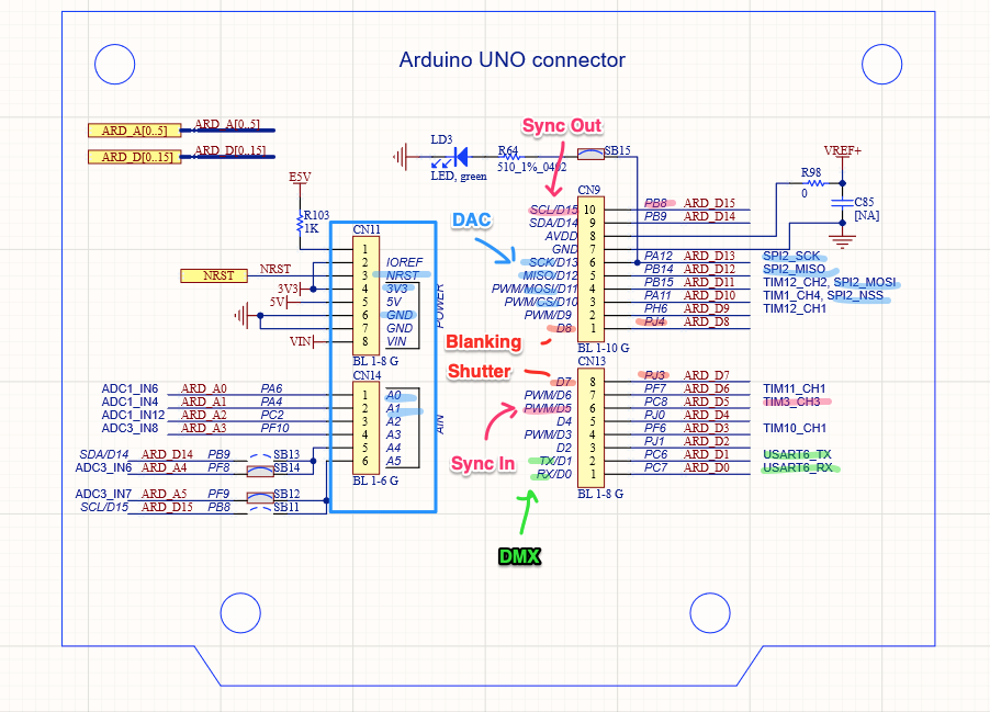
Four of the signals are for SPI and you might recognize them from the last post, but we are going to also make 5 additional connections:
The extra signals are 3.3V and GND from our controller board, the reset signal (NRST) to reset the DAC when our MCU resets, and two additional GPIO lines. These last two aren’t strictly necessary, but they give us access to the /CLR and /LDAC functions. /CLR immediately sets all DACs back to 0V and /LDAC can be used to “Load DACs” with a new value simultaneously. Our test connection looks like this:
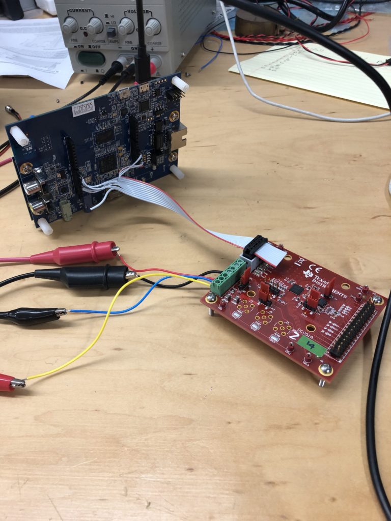
I already had used this DAC for a work project, so getting the SPI communication working with our EVAL board went pretty quickly. I ended up using the DAC in “Streaming Mode”:
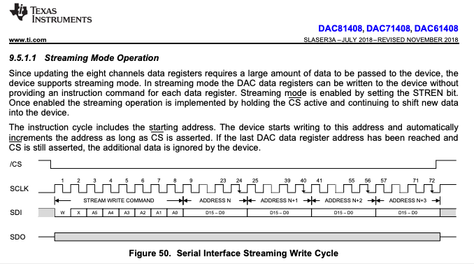
This writes all the DAC values in a single SPI transaction, with all the DACs updating when the /CS line goes high again (or, alternately, when we trigger the /LDAC line). Doing all the writes in a single transaction eliminates the wasted firmware overhead. But what about settle time?
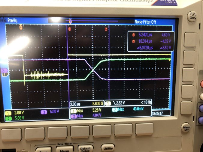
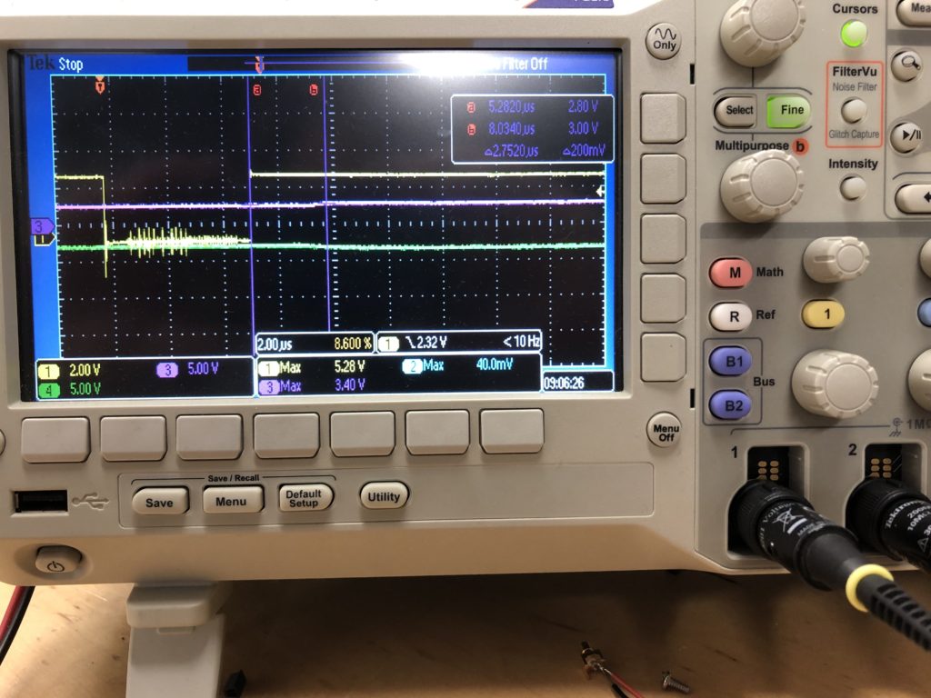
When it doubt, measure it. When operating in the +/-5V range we need for scanning, a full range jump settles in just over 5 uS in both directions (see the scope image at the top of this post). For smaller steps (1/32 of range), it is just under 3 uS:
That’s promising, but the real test is driving actual scanners. You might recall that the ILDA projector spec calls for a “differential signal”, not just X and Y, but X+ and X-, Y+ and Y-. As it happens, this DAC has a differential mode, where a second DAC channel can be set to automatically output the inverse of another. We most likely wouldn’t use this in a final design, since there are much cheaper ways to make a differential output, but it means that we are theoretically just a cable and some programming away from testing the DAC out for real.
This brought up a question of what to scan? Fortunately, ILDA has a specification for exchanging laser graphics. But it appears to be less well supported than one would hope (we’ll save that for a later post). A quick web search turned up a few pages with free-for-non-commercial-use ILDA graphics files, like this one.
With some ILDA files in hand, the next step was to read them and convert the data into something we could quickly put into firmware to test. We’re going to come back to this and write some nice, platform independent code in C++ for managing ILDA files on Mac, Windows, and Linux but, for a quick fix, I wrote two scripts in Matlab.
I wanted these anyway because Matlab already has 3D plotting and is a great platform to test all the matrix math operations that we’ll be adding later. I’ll post the scripts to a git repo in a day or so. I just want to add an “as-is, screw you if it doesn’t work or breaks anything” disclaimer first. [EDIT: More info and a link to the repo can be found here.] Anyway, the two scripts are pretty simple. First:
function [offsets fpath] = FindIldaFrames (inputfile)
% Find the offset of all the ILDA frames in an .ild file
% The inputfile can be omitted and the script will open a file selector
% Outputs a Nx1 matrix of offsets and (optional) the full path of the file parsed 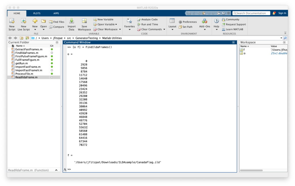
In this case ([o f] = FindIldaFrames()), we got two variables o, with the 25 offsets to frames in the file selected, and f, the full path to the CanadaFlag.ild file parsed (courtesy of function [offsets fpath] = FindIldaFrames (inputfile)). The second script gets the important data:
function [x y z s c] = ReadIldaFrame (inputfile, offset)
% Extract the X, Y, Z, status, and color information from a frame in an ILDA file
% If the inputfile is not provided a file selector dialog will appear
% Outputs the data in Nx1 matrices, except color (c), which can either be
% Nx1 if the file uses color indexes or Nx3 (R G B) if true color is used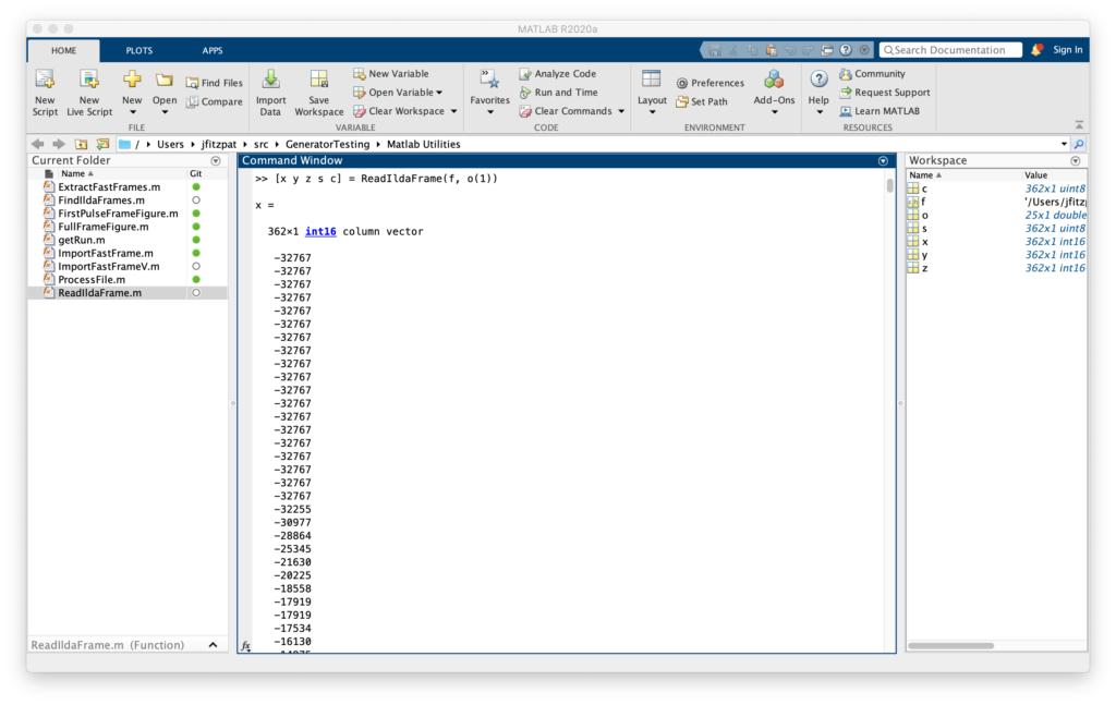
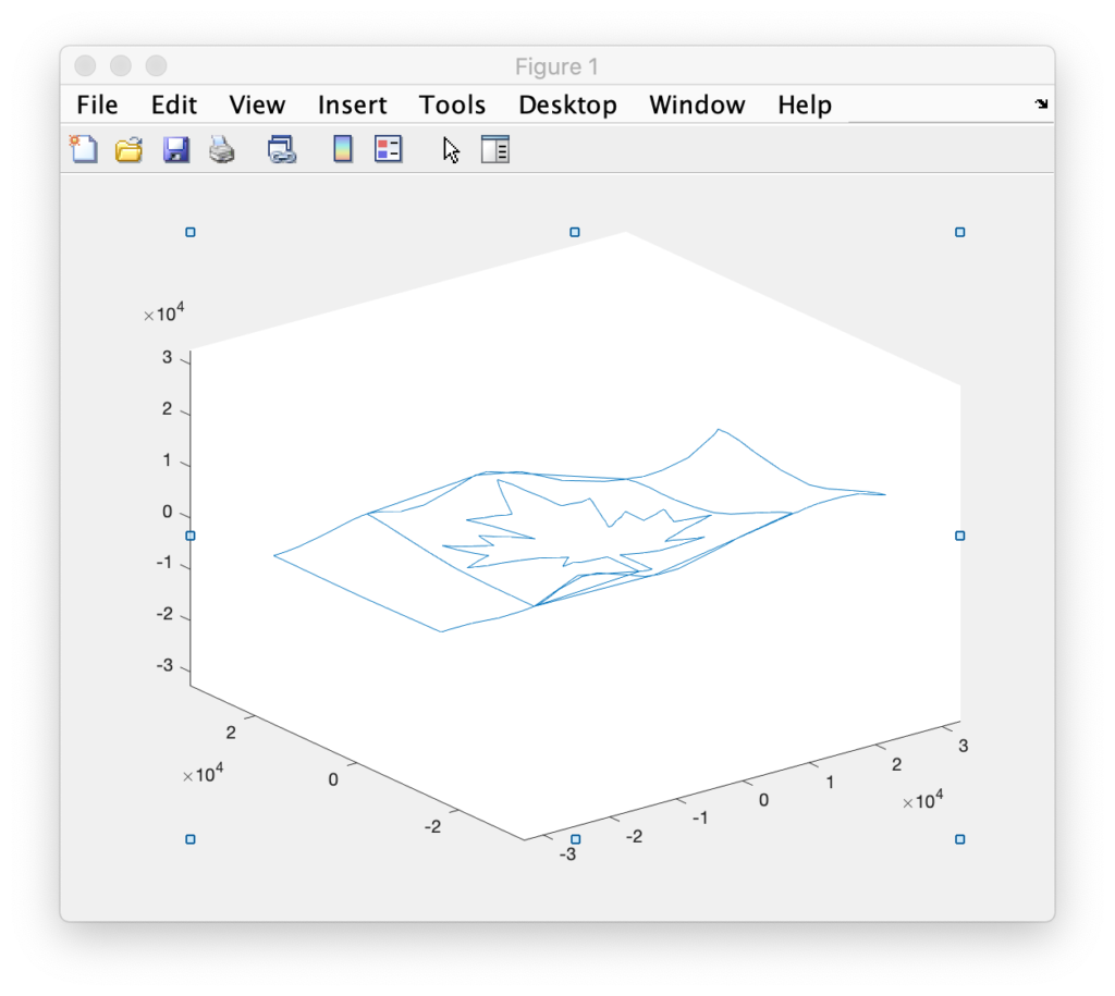
In this case ([x y z s c] = ReadIldaFrame(f, o(1))), got us all the data for the first frame of the file we parsed in the previous operation into some new variables. Entering plot3(x,y,z) will then show us, yep, it’s a Canadian flag drawn in 3D, we can rotate around:
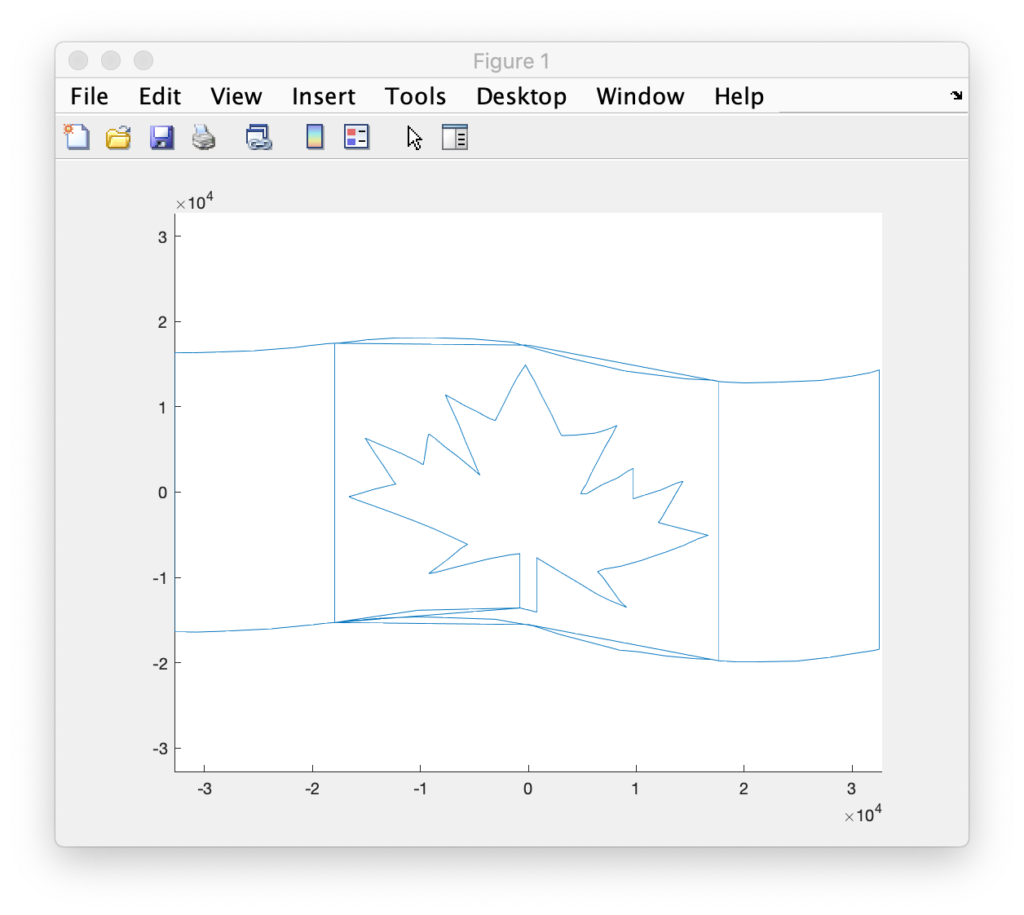
But we are seeing points and connections that are supposed to be ‘blanked’, or invisible. We can quickly distinguish the two using the status data we extracted. The status byte tells us one of two things, if a point is blanked, or if it is the last point in the frame. Entering:
>> blanked = s & 64;
>> visible = ~blanked;
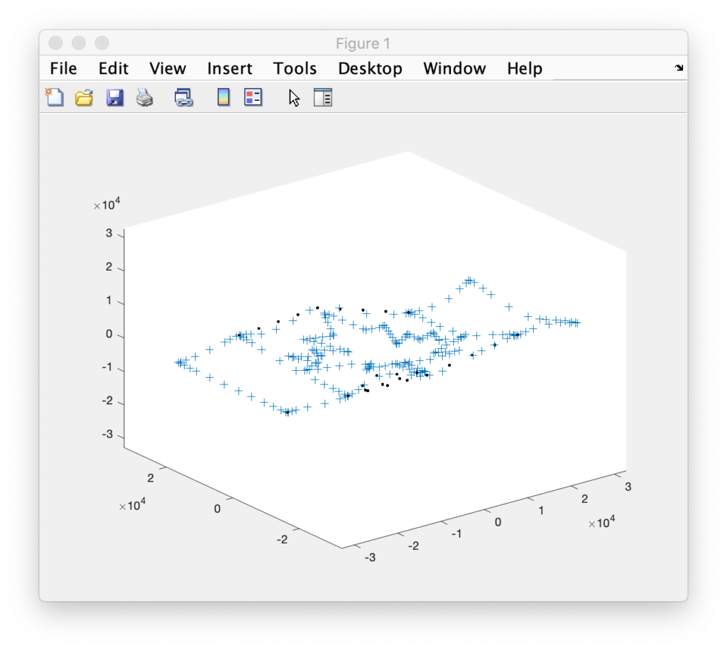
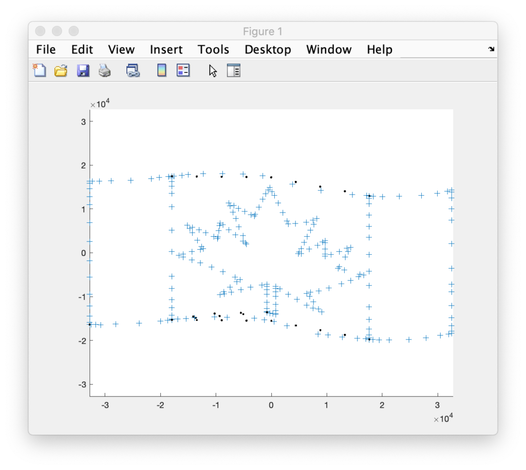
>> plot3(x(visible), y(visible), z(visible));
>> hold on;
>> plot3(x(blanked), y(blanked), z(blanked));Will plot the blanked and unblanked parts of the frame in different colors. It also can be helpful to change the graph to view everything as dots:
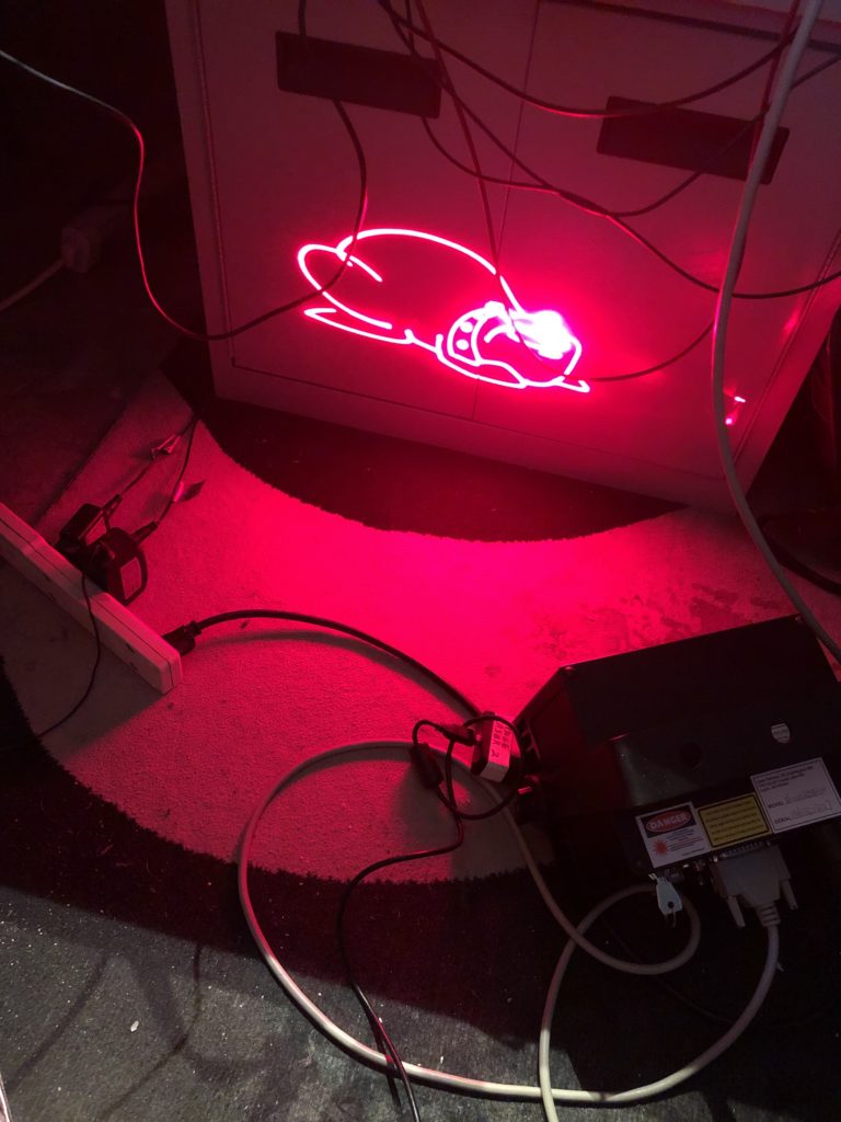
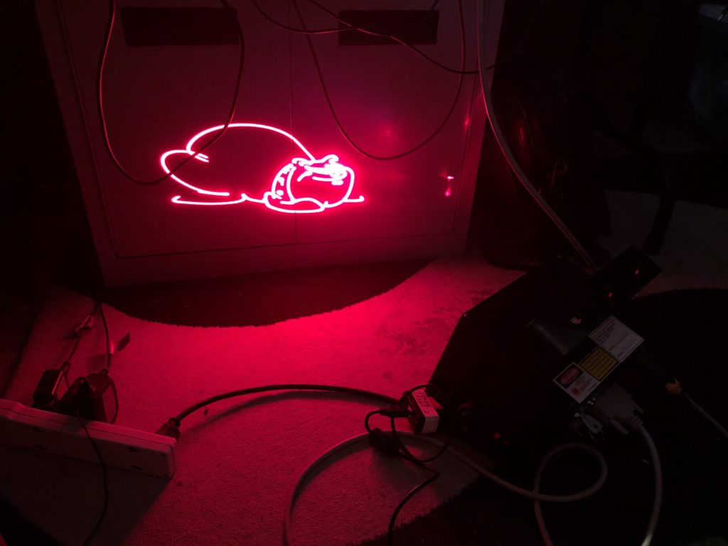
I was all set to do the scan test with a Canadian flag until Marty Canavan at YLS Entertainment sent me some vintage graphics as ILDA files. One of them being good ‘ol BULLDOG!
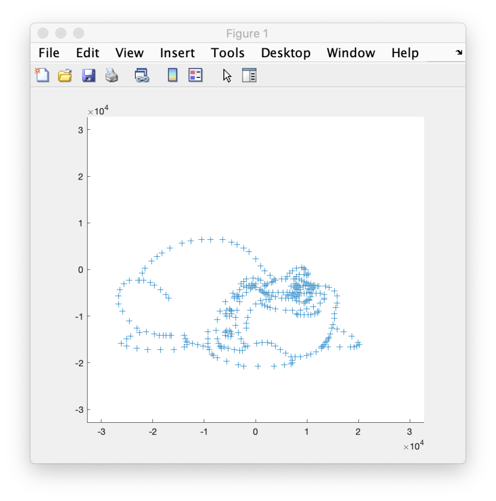
BULLDOG is actually an 8 frame animation, of which this is just one frame. It doesn’t look like much plotted this way, but it has always looked great as a scanned laser image. It was made during LaserMedia’s heyday, when the company employed artists and animators from Disney. They factored in how the scanners behaved in terms of inertia, etc. Alas, I can’t remember the particular artist’s name, but I distinctly remember using this animation when it was brand new. So, of course, it has to be the one!
Getting the data from Matlab to the compiler for our Eval board was easy. I used dlmwrite() to create comma delimited text files with the data and then included them in a C++ source file like this:
const int16_t dogX[] = {
#include "dogX.inc"
};

const int16_t dogY[] = {
#include "dogY.inc"
};

const uint8_t dogS[] = {
#include "dogS.inc"
};
Putting the image data in flash memory. Z data was all 0s and color data was all white, so I didn’t bother putting them in for this test drive. I setup a timer to scan the data and everything looked good, out to 60 kHz on the oscilloscope:
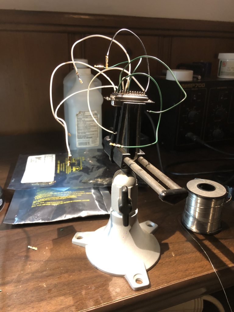
So I threw together a super kludgy DB-25 wire harness (reminiscent of a spider in honor of the lab mascot who came with the loaned projector):
Set the scan rate down to 14 kHz (what the image was originally drawn for), and hooked up the laser projector:
The rolling shutter really messes with our image (we’ll get to that!), but in person BULLDOG still looks great. If you futz with exposure and focus you can usually capture the whole image, but you lose all the details in the eyes, face, etc. that make the graphic so likeable:
One other thing worth pointing out is what happens when you increase scan speed. This projector is rated to 30 kHz. So I scanned the same image at 20 kHz, 25 kHz, and 30 kHz. The image doesn’t really distort, but what is visible and what is invisible shifts:
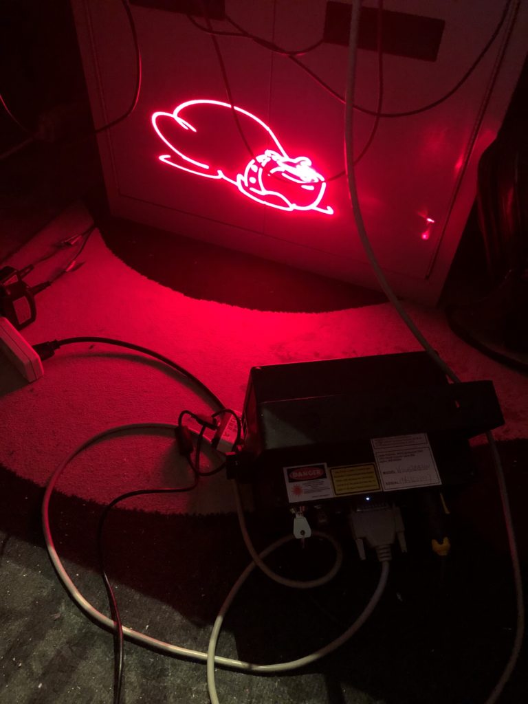
This is because the diode laser does not turn on and off instantly. We’ll address this down the road.
Next we will be back on our proper schematic and PCB, or maybe not!
Leave a Reply